Robust backfitting

Matias Salibian 2021-03-22

A robust backfitting algorithm

The R package RBF (available on CRAN here) implements the robust back-fitting algorithm as proposed by Boente, Martinez and Salibian-Barrera in

Boente G, Martinez A, Salibian-Barrera M. (2017) Robust estimators for additive models using backfitting. Journal of Nonparametric Statistics. Taylor & Francis; 29, 744-767. DOI: 10.1080/10485252.2017.1369077

This repository contains a development version of RBF which may differ slightly from the one available on CRAN (until the CRAN version is updated appropriately).

The package in this repository can be installed from within R by using the following code (assuming the devtools) package is available:

devtools::install_github("msalibian/RBF")

An example

Here is a (longish) example on how RBF works. We use the Air Quality data. The interest is in predicting Ozone in terms of three explanatory variables: Solar.R, Wind and Temp:

library(RBF)
data(airquality)
pairs(airquality[, c('Ozone', 'Solar.R', 'Wind', 'Temp')], 
      pch=19, col='gray30', cex=1.5)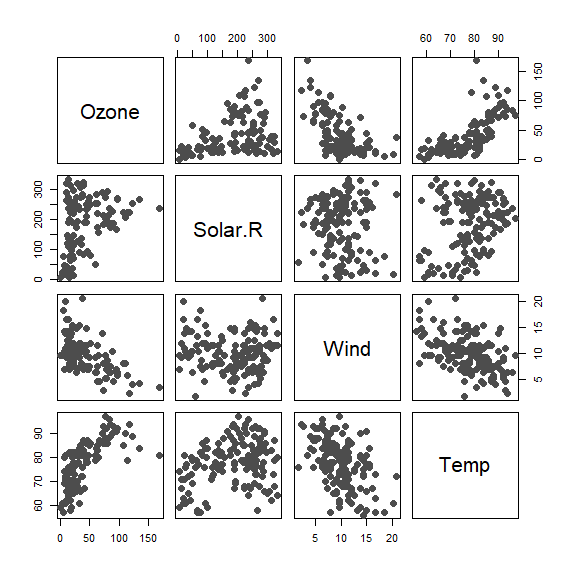

The following bandwidths were obtained via a robust leave-one-out cross-validation procedure (described in the paper). As a robust prediction error measure we use mu^2 + sigma^2 where mu and sigma are M-estimators of location and scale of the prediction errors, respectively. The code is copied below:

# Bandwidth selection with leave-one-out cross-validation
## Without outliers
# This takes a long time to compute (approx 380 minutes running
# R 3.6.1 on an Intel(R) Core(TM) i7-4790 CPU @ 3.60GHz)
ccs <- complete.cases(airquality)
x <- as.matrix( airquality[ccs, c('Solar.R', 'Wind', 'Temp')] )
y <- as.vector( airquality[ccs, 'Ozone'] )
a <- c(1/2, 1, 1.5, 2, 2.5, 3)
h1 <- a * sd(x[,1])
h2 <- a * sd(x[,2])
h3 <- a * sd(x[,3])
hh <- expand.grid(h1, h2, h3)
nh <- nrow(hh)
rmspe <- rep(NA, nh)
jbest <- 0
cvbest <- +Inf
# leave-one-out
n <- nrow(x)
for(i in 1:nh) {
  # leave-one-out CV loop
  preds <- rep(NA, n)
  for(j in 1:n) {
    tmp <- try( backf.rob(y ~ x, point = x[j, ],
                          windows = hh[i, ], epsilon = 1e-6,
                          degree = 1, type = 'Tukey', subset = c(-j) ))
    if (class(tmp)[1] != "try-error") {
      preds[j] <- rowSums(tmp$prediction) + tmp$alpha
    }
  }
  pred.res <- preds - y
  tmp.re <- RobStatTM::locScaleM(pred.res, na.rm=TRUE)
  rmspe[i] <- tmp.re$mu^2 + tmp.re$disper^2
  if( rmspe[i] < cvbest ) {
    jbest <- i
    cvbest <- rmspe[i]
    print('Record')
  }
  print(c(i, rmspe[i]))
}
bandw <- hh[jbest,]

Here we just set them to their optimal values:

bandw <- c(136.7285, 10.67314, 4.764985)

Now we use the robust backfitting algorithm to fit an additive model using Tukey’s bisquare loss (the default tuning constant for this loss function is 4.685). We remove cases with missing entries.

ccs <- complete.cases(airquality)
fit.full <- backf.rob(Ozone ~ Solar.R + Wind + Temp, data=airquality,
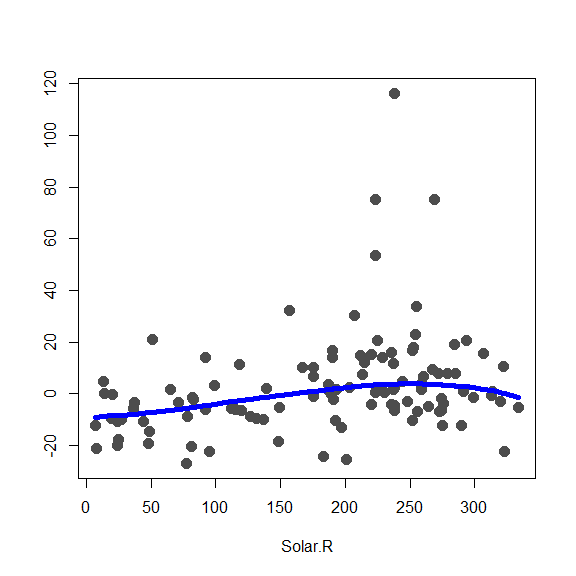
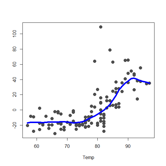
                subset=ccs, windows=bandw, degree=1, type='Tukey')

We display the 3 fits (one per additive component), being careful with the axis limits (which are stored to use them later):

lim.cl <- lim.rob <- matrix(0, 2, 3)
x0 <- fit.full$Xp
for(j in 1:3) {
  re <- fit.full$y - fit.full$alpha - rowSums(fit.full$g.matrix[,-j])
  lim.rob[,j] <- c(min(re), max(re))
  plot(re ~ x0[,j], type='p', pch=19, col='gray30', 
       xlab=colnames(x0)[j], ylab='', cex=1.5)
  oo <- order(x0[,j])
  lines(x0[oo,j], fit.full$g.matrix[oo,j], lwd=5, col='blue')
}

NOTE: These plots could also be obtained using the plot method:

# Plot each component
plot(fit.full, which=1:3)

We now compute and display the classical backfitting fits, with bandwidths chosen via leave-one-out CV:

library(gam)
x <- aircomplete[, c('Ozone', 'Solar.R', 'Wind', 'Temp')]
a <- c(.3, .4, .5, .6, .7, .8, .9)
hh <- expand.grid(a, a, a)
nh <- nrow(hh)
jbest <- 0
cvbest <- +Inf
n <- nrow(x)
for(i in 1:nh) {
  fi <- rep(0, n)
  for(j in 1:n) {
    tmp <- gam(Ozone ~ lo(Solar.R, span=hh[i,1]) + lo(Wind, span=hh[i,2])
               + lo(Temp, span=hh[i,3]), data=x, subset=c(-j))
    fi[j] <- as.numeric(predict(tmp, newdata=x[j,], type='response'))
  }
  ss <- mean((x$Ozone - fi)^2)
  if(ss < cvbest) {
    jbest <- i
    cvbest <- ss
  }
  print(c(i, ss))
}
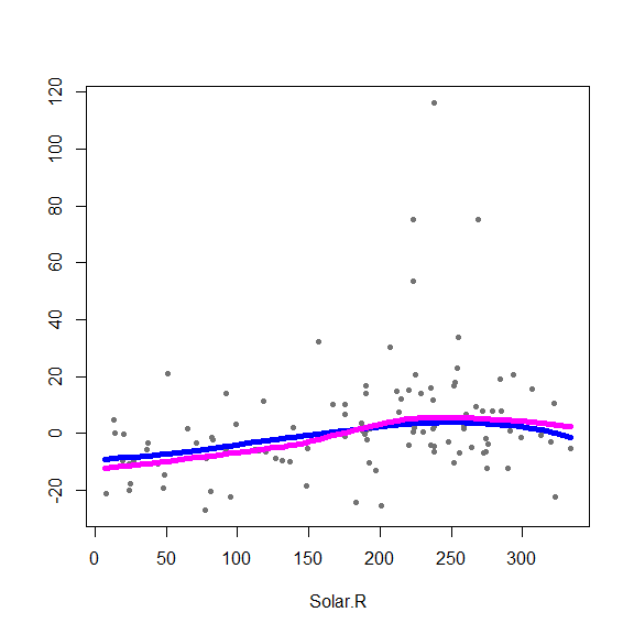
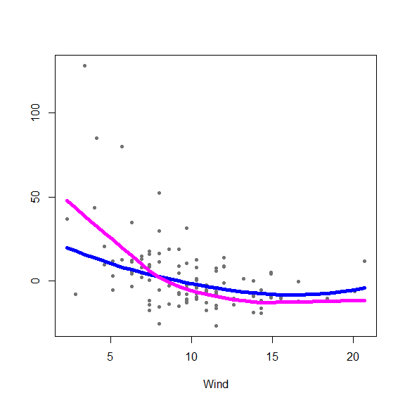
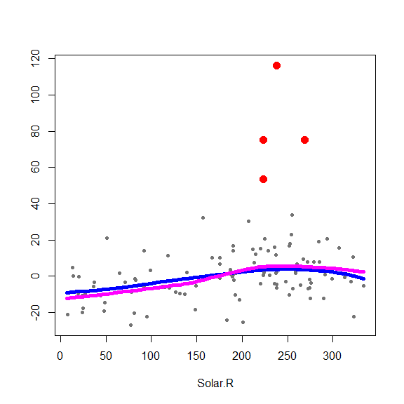
(hh[jbest,])

The optimal bandwidths are 0.7, 0.7 and 0.5 for Solar.R, Wind and Temp, respectively. Below are plots of partial residuals with the classical and robust fits overlaid:

aircomplete <- airquality[ complete.cases(airquality), ]
library(gam)
fit.gam <- gam(Ozone ~ lo(Solar.R, span=.7) + lo(Wind, span=.7)+
                 lo(Temp, span=.5), data=aircomplete)
# Plot both fits (robust and classical) 
x <- as.matrix( aircomplete[ , c('Solar.R', 'Wind', 'Temp')] )
y <- as.vector( aircomplete[ , 'Ozone'] )
fits <- predict(fit.gam, type='terms')
# alpha.gam <- attr(fits, 'constant')
for(j in 1:3) {
  re <- fit.full$yp - fit.full$alpha - rowSums(fit.full$g.matrix[,-j])
  plot(re ~ x[,j], type='p', pch=20, col='gray45', xlab=colnames(x)[j], ylab='')
  oo <- order(x[,j])
  lines(x[oo,j], fit.full$g.matrix[oo,j], lwd=5, col='blue')
  lines(x[oo,j], fits[oo,j], lwd=5, col='magenta')
}

To identify potential outiers we look at the residuals from the robust fit, and use the function boxplot:

re.ro <- residuals(fit.full)
ou.ro <- boxplot(re.ro, col='gray80')$out
in.ro <- (1:length(re.ro))[ re.ro %in% ou.ro ]
points(rep(1, length(in.ro)), re.ro[in.ro], pch=20, cex=1.5, col='red')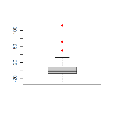

We highlight these suspicious observations on the scatter plot

cs <- rep('gray30', nrow(aircomplete))
cs[in.ro] <- 'red'
os <- 1:nrow(aircomplete)
os2 <- c(os[-in.ro], os[in.ro])
pairs(aircomplete[os2, c('Ozone', 'Solar.R', 'Wind', 'Temp')], 
      pch=19, col=cs[os2], cex=1.5)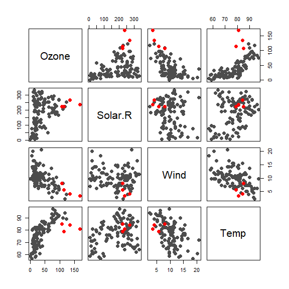

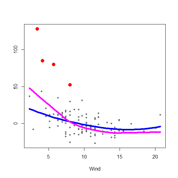
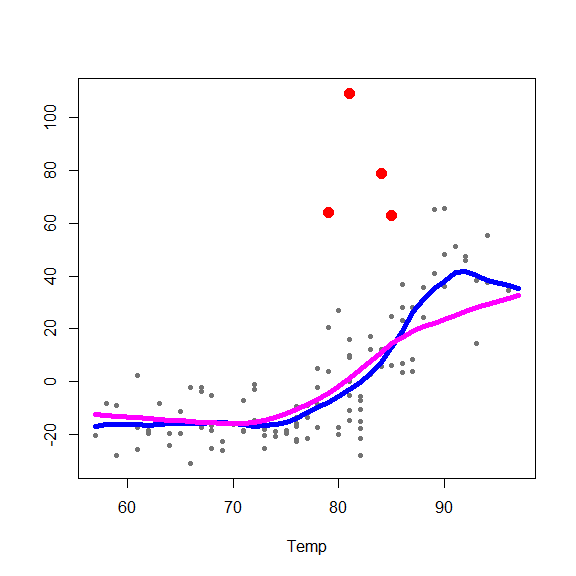
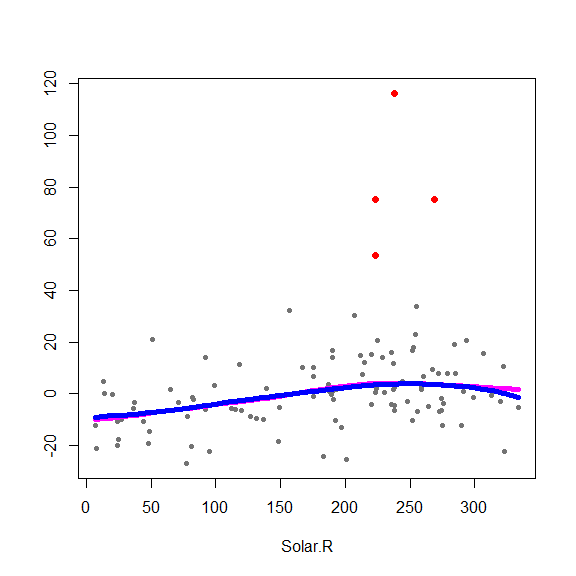
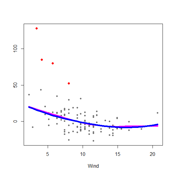
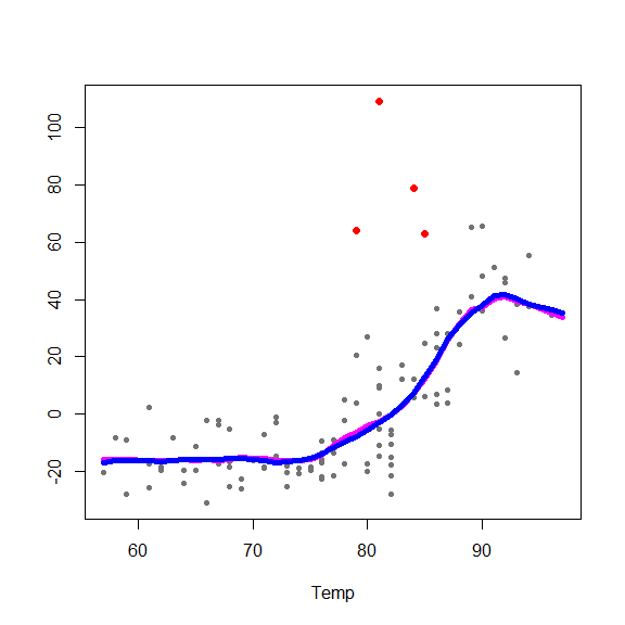
and on the partial residuals plots

for(j in 1:3) {
  re <- fit.full$yp - fit.full$alpha - rowSums(fit.full$g.matrix[,-j])
  plot(re ~ x[,j], type='p', pch=20, col='gray45', xlab=colnames(x)[j], ylab='')
  points(re[in.ro] ~ x0[in.ro,j], pch=19, col='red', cex=1.5)
  oo <- order(x[,j])
  lines(x[oo,j], fit.full$g.matrix[oo,j], lwd=5, col='blue')
  lines(x[oo,j], fits[oo,j], lwd=5, col='magenta')
}

We now compute the classical backfitting algorithm on the data without the potential outliers identified by the robust fit (the optimal smoothing parameters for the non-robust fit were re-computed using leave-one-out cross-validation on the “clean” data set). Note that now both fits (robust and non-robust) are
almost identical.

# Run the classical backfitting algorithm without outliers
airclean <- aircomplete[-in.ro, ]
fit.gam2 <- gam(Ozone ~ lo(Solar.R, span=.7) + lo(Wind, span=.8)+
                  lo(Temp, span=.3), data=airclean)
fits2 <- predict(fit.gam2, type='terms')
# alpha.gam2 <- attr(fits2, 'constant')
dd2 <- aircomplete[-in.ro, c('Solar.R', 'Wind', 'Temp')]
for(j in 1:3) {
  re <- fit.full$yp - fit.full$alpha - rowSums(fit.full$g.matrix[,-j])
  plot(re ~ x[,j], type='p', pch=20, col='gray45', xlab=colnames(x)[j], ylab='')
  points(re[in.ro] ~ x[in.ro,j], pch=20, col='red', cex=1.5)
  oo <- order(dd2[,j])
  lines(dd2[oo,j], fits2[oo,j], lwd=5, col='magenta')
  oo <- order(x[,j])
  lines(x[oo,j], fit.full$g.matrix[oo,j], lwd=5, col='blue')
}

Finally, we compare the prediction accuracy obtained with each of the fits. Because we are not interested in predicting well any possible outliers in the data, we evaluate the quality of the predictions using a 5%-trimmed mean squared prediction error (effectively measuring the prediction accuracy on 95% of the data). We use this alpha-trimmed mean squared function:

tms <- function(a, alpha=.1) {
  # alpha is the proportion to trim
  a2 <- sort(a^2, na.last=NA)
  n0 <- floor( length(a) * (1 - alpha) )
  return( mean(a2[1:n0], na.rm=TRUE) )
}

We use 100 runs of 5-fold CV to compare the 5%-trimmed mean squared prediction error of the robust fit and the classical one. Note that the bandwidths are kept fixed at their optimal value estimated above.

dd <- airquality
dd <- dd[complete.cases(dd), c('Ozone', 'Solar.R', 'Wind', 'Temp')]
# 100 runs of K-fold CV
M <- 100
# 5-fold
K <- 5
n <- nrow(dd)
# store (trimmed) TMSPE for robust and gam, and also
tmspe.ro <- tmspe.gam <- vector('numeric', M)
set.seed(123)
ii <- (1:n)%%K + 1
for(runs in 1:M) {
  tmpro <- tmpgam <- vector('numeric', n)
  ii <- sample(ii)
  for(j in 1:K) {
    fit.full <- backf.rob(Ozone ~ Solar.R + Wind + Temp, 
                           point=dd[ii==j, -1], windows=bandw, 
                           epsilon=1e-6, degree=1, type='Tukey', 
                           subset = (ii!=j), data = dd)
    tmpro[ ii == j ] <- rowSums(fit.full$prediction) + fit.full$alpha
    fit.gam <- gam(Ozone ~ lo(Solar.R, span=.7) + lo(Wind, span=.7)+
                     lo(Temp, span=.5), data=dd[ii!=j, ])
    tmpgam[ ii == j ] <- predict(fit.gam, newdata=dd[ii==j, ], type='response')
  }
  tmspe.ro[runs] <- tms( dd$Ozone - tmpro, alpha=0.05)
  tmspe.gam[runs] <- tms( dd$Ozone - tmpgam, alpha=0.05)
}

These are the boxplots. We see that the robust fit consistently fits the vast majority (95%) of the data better than the classical one.

boxplot(tmspe.ro, tmspe.gam, names=c('Robust', 'Classical'), 
        col=c('tomato3', 'gray80')) #, main='', ylim=c(130, 210))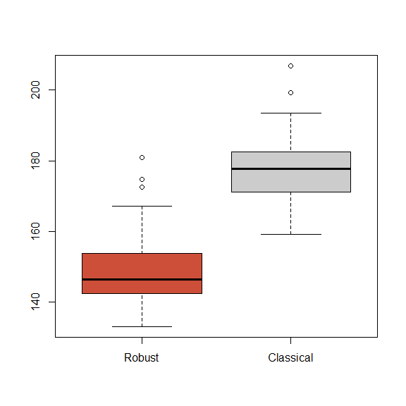

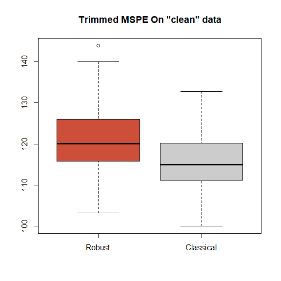
As a sanity check, we compare the prediction accuracy of the robust and non-robust fits using only the “clean” data set. We re-compute the optimal bandwidths for the robust fit using leave-one-out cross validation as above, and as above, note that these bandwidths are kept fixed. We use 100 runs of 5-fold cross-validation, and compute both the trimmed and the regular mean squared prediction errors of each fit.

aq <- airquality
aq2 <- aq[complete.cases(aq), c('Ozone', 'Solar.R', 'Wind', 'Temp')]
airclean <- aq2[ -in.ro, ]
bandw <- c(138.2699, 10.46753, 4.828436)
M <- 100 
K <- 5
n <- nrow(airclean)
mspe.ro <- mspe.gam <- tmspe.ro <- tmspe.gam <- vector('numeric', M)
set.seed(17)
ii <- (1:n)%%K + 1
for(runs in 1:M) {
  tmpro <- tmpgam <- vector('numeric', n)
  ii <- sample(ii)
  for(j in 1:K) {
    fit.full <- try( backf.rob(Ozone ~ Solar.R + Wind + Temp, 
                          point=airclean[ii==j, -1], windows=bandw, 
                          epsilon=1e-6, degree=1, type='Tukey', 
                          subset = (ii!=j), data = airclean) )
    if (class(fit.full)[1] != "try-error") {
      tmpro[ ii == j ] <- rowSums(fit.full$prediction) + fit.full$alpha
    }
    fit.gam <- gam(Ozone ~ lo(Solar.R, span=.7) + lo(Wind, span=.8)+
                     lo(Temp, span=.3), data=airclean, subset = (ii!=j) )
    tmpgam[ ii == j ] <- predict(fit.gam, newdata=airclean[ii==j, ], 
                                 type='response')
  }
  tmspe.ro[runs] <- tms( airclean$Ozone - tmpro, alpha=0.05)
  mspe.ro[runs] <- mean( ( airclean$Ozone - tmpro)^2, na.rm=TRUE)
  tmspe.gam[runs] <- tms( airclean$Ozone - tmpgam, alpha=0.05)
  mspe.gam[runs] <- mean( ( airclean$Ozone - tmpgam)^2, na.rm=TRUE)
}

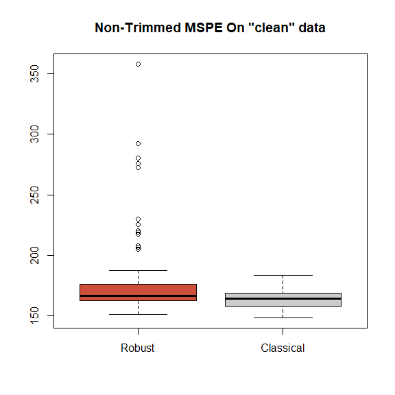
The boxplots of the trimmed and regular mean squared prediction errors over the 100 cross-validation runs are below. We see that for the majority of the runs both estimators provide very similar prediction errors. Note that we naturally expect a robust method to perform slightly worse than the classical one when no model deviations occur. The boxplots below show that for this robust backfitting estimator, this loss in prediction accuracy is in fact very small.

boxplot(tmspe.ro, tmspe.gam, names=c('Robust', 'Classical'), 
        col=rep(c('tomato3', 'gray80'), 2), main='Trimmed MSPE On "clean" data')
boxplot(mspe.ro, mspe.gam, names=c('Robust', 'Classical'), 
        col=rep(c('tomato3', 'gray80'), 2), main='Non-Trimmed MSPE On "clean" data')